Learning with various rule-based models and model selection strategies

This tutorial will walk you through an application of Kover to a set of genomes labelled according to their phenotypes. We use data from the paper (see data), but you could use your own. Specifically, we will use the CART and SCM algorithms to learn models that predict Azithromycin resistance in Neisseria gonorrhoeae.

For an introduction to machine learning , please refer to this tutorial.

Getting the example Kover dataset

First download the pre-created dataset (~100 Mb) which contains the genome of 392 Neisseria gonorrhoeae isolates, along with their susceptibility to Azithromycin. Next, unzip the file and then change into the resulting directory.

cd kover-example

The file “example.kover” is the Kover dataset which use a compressed and optimized representation of the data (details here).

Exploring the dataset

You can use the kover dataset info command to print information about the dataset. For example, to print the number of genomes and k-mers in the dataset, use:

kover dataset info --dataset example.kover --genome-count --kmer-count

Your dataset contains 392 genomes vs. 4 766 702 k-mers! Notice that the number of genomes is significantly smaller than the number of k-mers. In machine learning, this is known as fat data and is particularly challenging for learning algorithms. Fortunately, Kover is very efficient at learning from this kind of data.

Splitting the data into training and testing sets

In order to measure the accuracy of models obtained using Kover, we must split the data into a training set and a validation set. The training set will be used to learn models and the validation set will be used to measure their accuracy. A Kover dataset can contain multiple splits of the data, which are created using the kover dataset split command.

Furthermore, the algorithms implemented in Kover have hyperparameters, which are parameters that control the behavior of the algorithm and must be manually set by the user. Selecting the value of such parameters is known as model selection. Kover implements two model selection strategies: k-fold cross-validation and bound selection. k-fold cross-validation is the most expensive and it requires that small partitions of the data, called folds be created. Bound selection is considerably faster and does not require the creation of such folds.

The following command creates a split of the data called “example_split”, which uses 80% of the genomes for training and 20% for testing. It also creates 10 cross-validation folds. The data are partitioned randomly, using 2 as the random seed.

kover dataset split --dataset example.kover --id example_split --train-size 0.80 --folds 10 --random-seed 2 --progress

Note: You can set --folds 0 if you will only be using bound selection.

Learning models

Now that we have created and splitted the dataset, we are ready to learn predictive model of Azithromcycin resistance in Neisseria gonorrhoeae. The kover learn command is used to learn models for Set Covering Machines and Classficication and Regression Trees.

Set Covering Machines

Let start by training the Set Covering Machine algorithm on this dataset. We will try the following values for the hyperparameters:

• Maximum number of rules in the model: 10
• Type of model: conjunction (logical-AND) or disjunction (logical-OR)
• p (see documentation): 0.1, 1.0 and 10.0

Cross-Validation

The following command tells Kover to use the SCM algorithm and cross-validation as the model selection strategy. Moreover, it distributes the cross-validation on 4 CPUs and outputs the result files into the results/scm_cv directory.

kover learn scm --dataset example.kover --split example_split --model-type conjunction disjunction --p 0.1 1.0 10.0 --max-rules 10 --hp-choice cv --n-cpu 4 --output-dir results/scm_cv --progress

The total computation time is around 3 minutes. Kover then uses the obtained model to predict the phenotype of the genomes in the testing set and computes various metrics. For this example, the obtained model is:

Model (Conjunction - 3 rules):
------------------------------
Presence(AAACTTCCAACGCCCACTGCAGATAGGGACC) [Importance: 0.74, 62 equivalent rules]
AND
Absence(AGAGTCGTTGTCTTTGGGCCATTCGCCGTGA) [Importance: 0.17, 2 equivalent rules]
AND
Presence(ATTCGACTGTGCGTAAAAATCGTCCGCTACG) [Importance: 0.18, 7 equivalent rules]

Notice the simplicity and interpretability of the obtained model. The testing set metrics for this model are:

Error Rate: 0.08974
Sensitivity: 1.0
Specificity: 0.85106
Precision: 0.81579
Recall: 1.0
F1 Score: 0.89855
True Positives: 31.0
True Negatives: 40.0
False Positives: 7.0
False Negatives: 0.0

Bound selection

Let’s now use bound selection as the model selection strategy and compare it to cross-validation. We only have to modify the previous command to specify --hp-choice bound and output the result files in another directory, results/scm_b.

kover learn scm --dataset example.kover --split example_split --model-type conjunction disjunction --p 0.1 1.0 10.0 --max-rules 10 --hp-choice bound  --output-dir results/scm_b --progress

Using bound selection, the computation time drop to just under 20 seconds! The resulting model has the same number of rules, but relies on different k-mers.

Model (Conjunction - 3 rules):
------------------------------
Absence(AAGTGTTTTTGTTATAAAAACGCTGCCCGAA) [Importance: 0.85, 28 equivalent rules]
AND
Presence(AAACTTCCAACGCCCACTGCAGATAGGGACC) [Importance: 0.60, 62 equivalent rules]
AND
Absence(ACACGGGGATGAGTTTGAACAGGTCGGTTAC) [Importance: 0.19, 19 equivalent rules]

And the testing set metrics for this new model are:

Error Rate: 0.02564
Sensitivity: 1.0
Specificity: 0.95745
Precision: 0.93939
Recall: 1.0
F1 Score: 0.96875
True Positives: 31.0
True Negatives: 45.0
False Positives: 2.0
False Negatives: 0.0

As we can see, for this example, using bound selection instead of cross-validation requires less computation time and produces a more accurate model.

Classification and Regression Trees

Let’s now learn a decision tree model using the Classification and Regression Tree algorithm. We will try the following values for the hyperparameters:

• Max depth: 20
• Minimum number of examples to split a leaf: 2
• Criterion: gini

Cross-Validation

The following command tells Kover to learn a tree model, using cross-validation as the model selection strategy. Moreover, it distributes the cross-validation on 4 CPUs and outputs the result files into the results/cart_cv directory.

kover learn tree --dataset example.kover --split example_split --criterion gini --max-depth 20 --min-samples-split 2 --hp-choice cv --n-cpu 4 --output-dir results/cart_cv --progress

The computation time is slightly under 5 minutes and the resulting tree model, which contains 12 rules and has a depth of 6, is textually represented in the report (results/cart_cv/report.txt). For a better visual representation, we can use the plot_model.py script, which should be present alongside the data:

Warning: The script assumes that LaTeX is installed on your computer.

python plot_model.py results/cart_cv/model.fasta

to obtain the following representation of the decision tree model:

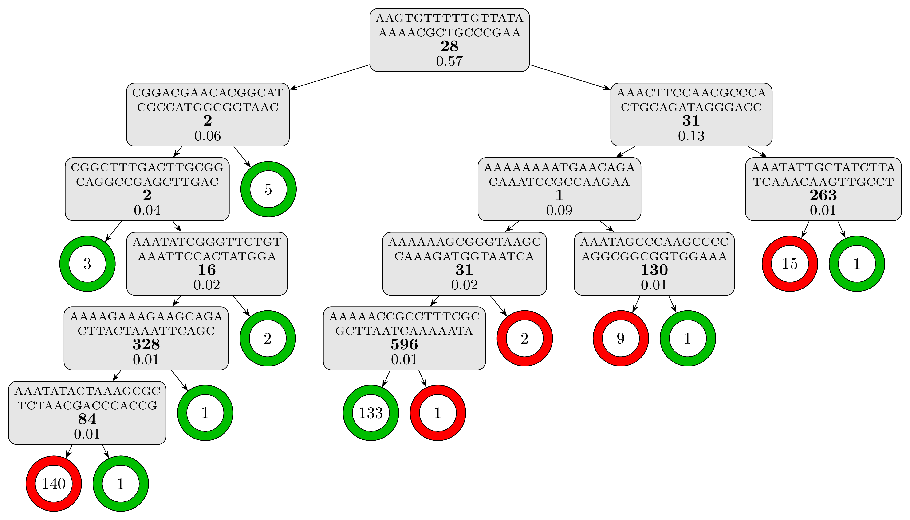
The testing set metrics for this model are:

Error Rate: 0.03846
Sensitivity: 1.0
Specificity: 0.93617
Precision: 0.91176
Recall: 1.0
F1 Score: 0.95385
True Positives: 31.0
True Negatives: 44.0
False Positives: 3.0
False Negatives: 0.0

Bound selection

Let’s now use bound selection as the model selection strategy and see how it affect the learning for CART. We only have to modify the previous command to specify --hp-choice bound and output the result files in another directory, results/cart_b.

kover learn tree --dataset example.kover --split example_split --criterion gini --max-depth 20 --min-samples-split 2 --hp-choice bound --n-cpu 4 --output-dir results/cart_b --progress

Using bound selection, the computation time drop to just under 25 seconds! The resulting model is a lot simpler with only 4 rules and a depth of 3. Using the same script, we can visualize the model:

python plot_model.py results/cart_b/model.fasta

we obtain this visual representation highlighting how simple and interpretable this model is:

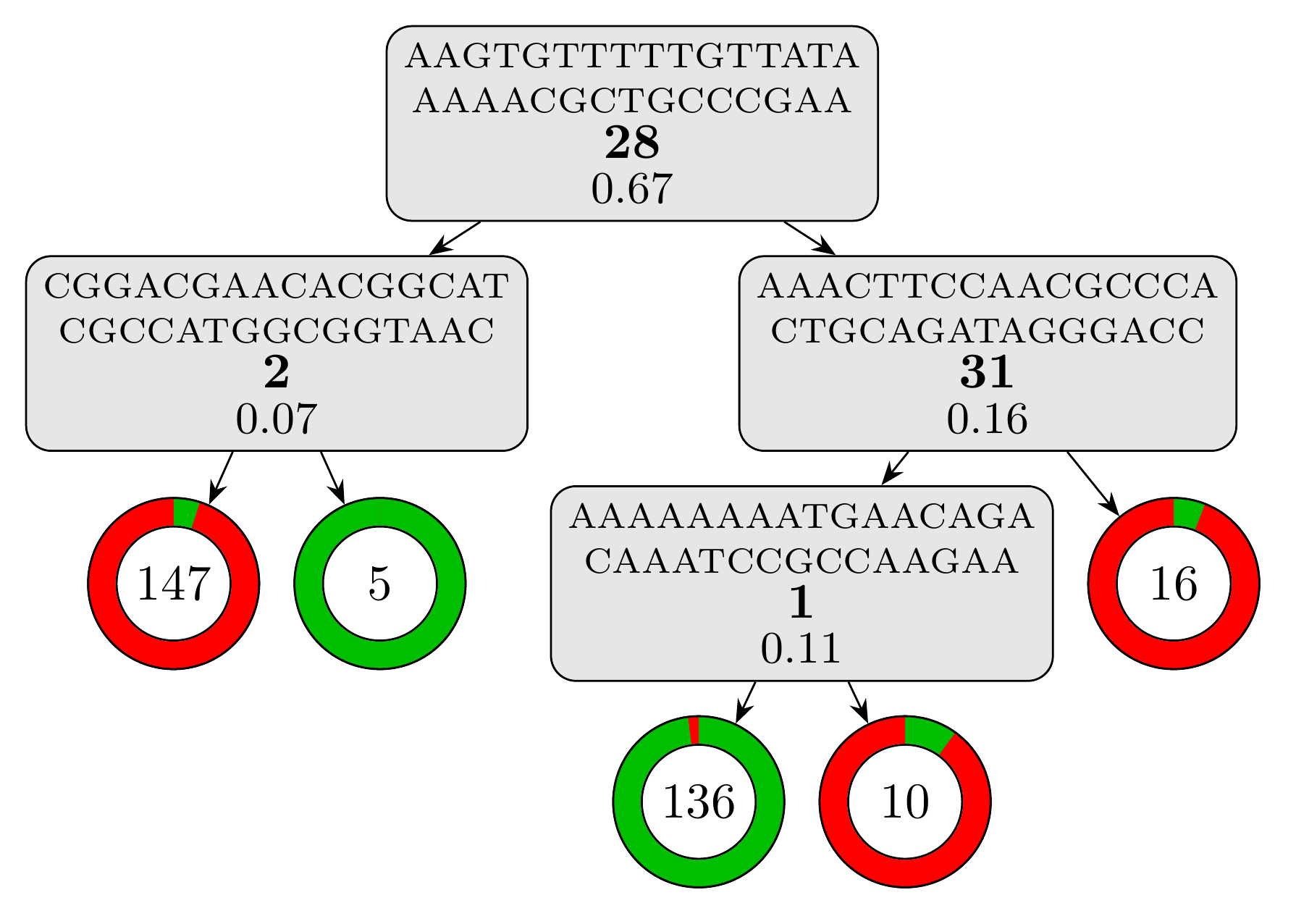
And the testing set metrics for this new model are:

Error Rate: 0.01282
Sensitivity: 1.0
Specificity: 0.97872
Precision: 0.96875
Recall: 1.0
F1 Score: 0.98413
True Positives: 31.0
True Negatives: 46.0
False Positives: 1.0
False Negatives: 0.0

That’s it! You know how to use Kover to learn rule-based genotype-to-phenotype models. Now, try it on your own data.

For a tutorial on interpreting the learned models using genome annotations, see here.